Variationnal approaches for image restoration
For the following exercices, you need Matlab. The subject of the following exercices is image restoration. All my thanks to Remy Abergel for his help during the realization of this course.
Sommaire
1 Introduction
- Write a function \([fx,fy]=grad(f)\) which takes as input an image \(f\) and computes the gradient of \(f\) using the following scheme $$ fx(i,j) = \begin{cases} f(i+1,j) - f(i,j) &\text{ if } i<n \\ 0 &\text{ else} \end{cases},\;\;\;\;\; fy(i,j) = \begin{cases} f(i,j+1) - f(i,j) &\text{ if } j<m \\ 0 &\text{ else.} \end{cases}$$ Note : if you use Matlab with the image processing toolbox, you can use the function 'imgradientxy' with the option 'IntermediateDifference'.
- Recall that the divergence of a function \(g:\mathbb{R}^2\rightarrow \mathbb{R}^2\) is defined as \(\mathrm{div}(g) = \frac{\partial g_x}{\partial x}+\frac{\partial g_y}{\partial y}\). Write a function \(d = div(gx,gy)\) which takes a vector field \(g=[gx,gy]\) (\(g\) is a \(n\times m\times 2\) matrix) and computes the divergence of the field using the following scheme :
$$div(g)_{(i,j)} = \begin{cases} gx(i,j) - gx(i-1,j) &\text{ if } 1<i<n \\ gx(i,j) &\text{ if } i=1 \\ -gx(i-1,j) &\text{ if } i=n \end{cases}+ \begin{cases} gy(i,j) - gy(i,j-1) &\text{ if } 1<j<n \\gy(i,j) &\text{ if } j=1 \\ -gy(i,j-1) &\text{ if } j=n \end{cases}$$
- Use the previous functions to write a function \(l = laplacien(f)\) which computes the laplacian of the discrete image \(f\) (recall that \(\Delta f = \mathrm{div}(\nabla f)\)).
2 Inpainting
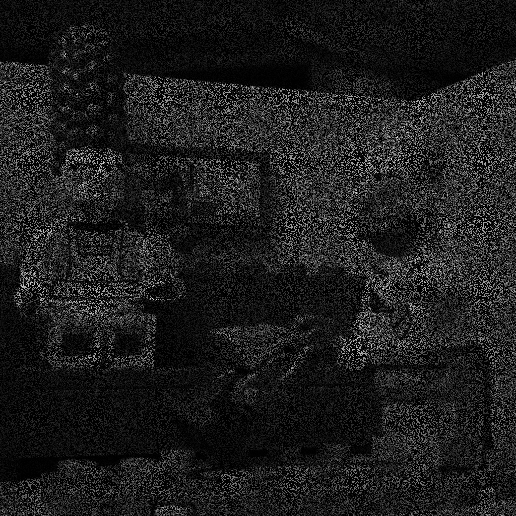
In the following, we assume that the values of a random set of pixels in the original image are missing, the goal is to interpolate the resulting image.
Creation of the degraded image :
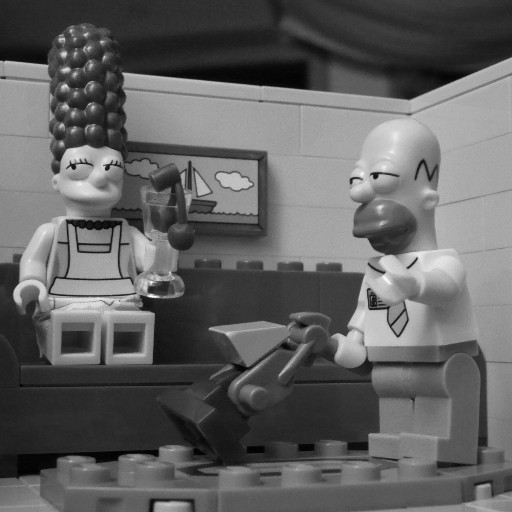
f = double(imread('simpson_nb512.png'));
f = f/max(f(:)); % normalization between 0 and 1 in order to fix parameters more easily
mask = (rand(size(f))>.7);   % mask creation
v = f.*mask  ;
figure(1);imshow(f); figure(2);imshow(v);
Be careful with the function imshow(). If u is an image encoded in double, imshow(u) will display all values above 1 in white and all values below 0 in black. If the image u is encoded on 8 bits though, imshow(u) will display 0 in black and 255 in white. In order to scale u and use the full colormap, use the command imshow(u,[]).
In order to interpolate \(v\), we propose to minimize the \(TV\)-based energy $$E(f) = \sum_{i=1}^n\sum_{j=1}^m \|(\nabla f)_{i,j}\|_2.$$ on the set \(C\) of images taking the same values as \(v\) outside of the mask.
To this aim, we can make use of a projected gradient descent : at each step of the gradient descent on \(E\), we reproject the result on the constraint \(\{u \in C\}\). The derivative of \(E\) can be written $$\frac{\partial E}{\partial f} = - \mathrm{div}\left(\frac{\nabla f }{\|\nabla f\|_2}\right),$$ and we can replace \(\|\nabla f\|_2\) by \(\sqrt{\|\nabla f\|_2^2 +\varepsilon^2}\) with a small \(\varepsilon\) to avoid division by \(0\).
u = v;
epsilon = 0.01;
p = 0.002;     % gradient step
N=2000           % number of iterations (try with a smaller number of iterations first)
for i = 1:N
 INSERT YOUR CODE HERE
end

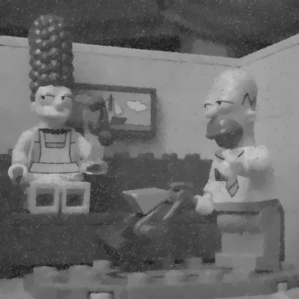
image interpolated with the previous method (applied on the 1024x1024 Simpson image with 70% of hidden pixels).
3 Denoising
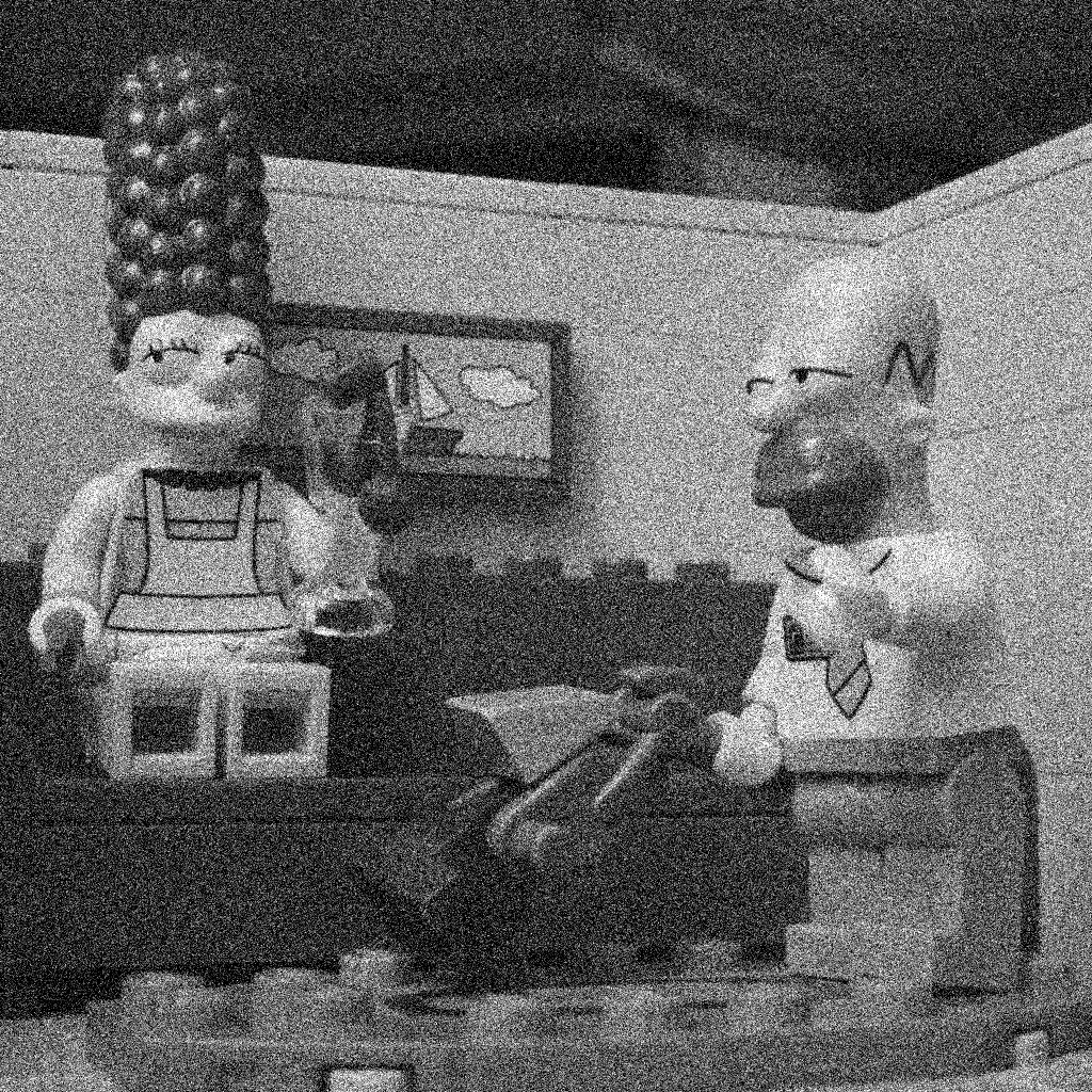
Create the noisy image.
f = double(imread('simpson_nb512.png'));
f = f/max(f(:)); % normalization between 0 and 1 in order to fix parameters more easily
ub = f + randn(size(f))*.2; % we add gaussian noise with std = 0.2
figure(1);imshow(f);figure(2);imshow(ub);
3.1 Tychonov
We propose to denoise \(u_b\) by finding \(u\) which minimizes $$E(u) = \frac{1}{2}\|u_b-u\|_2^2+\lambda \int |\nabla u|^2,$$ where \(|\nabla u|\) denotes the norm of \(\nabla u\) in \(\mathbb{R}^2\).
The formulation is convex, differentiable, so we can apply a gradient descent scheme with $$\frac{\partial E}{\partial u} =(u-u_b)-2\lambda\Delta u.$$
p = 0.01; % gradient step
N = 100; % number of iterations
lambda = 5;
u = ub;
for k=1:N
    deltau = laplacien(u);
    u = u - p*(u-ub-2*lambda*deltau);
end
figure(3);imshow(u,[]);colormap gray;

You can also observe how the energy \(E\) decreases through the iterations.
3.2 TV-L2
The Laplacian operator in the previous model does not preserve edges correctly: the result is oversmoothed. In order to preserve edges, we can replace the \(L^2\) norm by a \(L^1\) norm in the regularization term. The energy becomes $$E(u) = \frac{1}{2}\|u_b-u\|_2^2+\lambda TV(u),$$ with \(TV(u)\) the discrete version of the total variation $$TV(u) =\sum_{(i,j)} |(\nabla u)_{i,j}|.$$ This energy is convex but not differentiable when \(\nabla u \neq 0\) at some points. If \(\nabla u \neq 0\) everywhere, then $$\frac{\partial E}{\partial u} =(u-u_b)-\lambda \mathrm{div} \frac{\nabla u}{\|\nabla u\|}.$$ In practice we can apply a gradient descente by approximating \(\|\nabla u\|\) by \(\sqrt{\|\nabla u\|^2+\varepsilon^2}\) with a small value \(\varepsilon\).
lambda = 0.5;
epsilon = 0.001;
p = 0.0005;
N = 2000;
u = ub;
for i = 1:N
    [ux,uy]  = grad(u);
    normgrad = sqrt(ux.^2+uy.^2+epsilon^2);
    u = u - p*(u-ub-lambda*div(ux./normgrad,uy./normgrad));
end
figure(3);imshow(u,[]);
Display the result and the energy \(E\) through the iterations. Unfortunately, the number of iterations necessary to converge is often prohibitive in practice, especially if \(\varepsilon\) is chosen very small. A more convenient algorithm is proposed in the next section.

3.3 TV-L1
In order to minimize the convex but non-smooth energy $$E(u) = \|u_b-u\|_1+\lambda TV(u),$$ we propose to make use of a primal-dual algorithm, designed to find solutions of (smooth or non smooth) convex problems of the form (see for instance (Chambolle-Pock, 2010)): $$\min_{u \in X} \max_{p \in X\times X} (Ku,p) + G(u) -F^*(p),$$ with \(K\) linear and \(G: X\rightarrow \mathbb{R}^+\) and \(F^*: X\rightarrow \mathbb{R}^+\) convex, proper, lower-semicontinuous.
It happens that $$TV(u) = \max_{p\in X\times X} <\nabla u, p >_X -\iota_{\kappa}(p),$$ where $$\iota_{\kappa}(p) = \begin{cases} 0 &\mbox{if } p\in \kappa\\ +\infty &\mbox{if } p\notin \kappa. \end{cases} \text{ and } \kappa = \{\mathrm{div} p \;/ \;\max_{x\in\Omega}|p(x)| \leq 1\}.$$ The TV-L1 problem can be written as a min-max under the previous form by choosing $$G(u) = \|u_b-u\|_1, \;\;F^*(p) =\iota_{\kappa}(p) \text{ and } K = \lambda \nabla (\text{ thus } K^* = -\lambda \mathrm{div})$$
The simple primal-dual algorithm we propose to use can be written
- Initialization : choose \(\tau\), \(\sigma >0\), \((u^0,p^0)\)
- Iterations for \(n\geq 0\) : \begin{cases} p^{n+1} &=& \underbrace{\mathrm{prox}_{\sigma F^*}}_{\text{backward step}} \underbrace{(p^n + \sigma K \bar{u}^n)}_{\text{forward step}} \\ u^{n+1} &=& \mathrm{prox}_{\tau G} (u^n-\tau K^* p^{n+1})\\ \bar{u}^{n+1} &=& u^{n+1} + \theta (u^{n+1} - u^n) \end{cases}
If \(\theta=0\), the previous scheme is semi-implicit : \(p^{n+1}\) is computed from \(p^n\) and \(u^n\), and \(u^{n+1}\) is computed from \(u^n\) and \(p^{n+1}\). In the last line, \(\bar{u}^{n+1}\) is a linear extrapolation, based on \(u^n\) and \(u^{n+1}\). It permits to make the scheme a little bit more implicit by using an updated value of \(u^{n}\) when computing \(p^{n+1}\).
Using the previous scheme makes sense because \(\mathrm{prox}_{\sigma F^*}\) and \(\mathrm{prox}_{\tau G}\) are easy to compute in the TV-L1 case : $$\left(\mathrm{prox}_{\tau G}(u)\right)_{i,j} = \begin{cases} u_{i,j} - \tau &\mbox{if } u_{i,j} - (u_b)_{i,j} > \tau \\ u_{i,j} + \tau &\mbox{if } u_{i,j} - (u_b)_{i,j} < \tau \\ (u_b)_{i,j} &\mbox{if } |u_{i,j} - (u_b)_{i,j}| \leq \tau \\ \end{cases}$$ $$\left(\mathrm{prox}_{\sigma F^*}(p)\right)_{i,j} = \left(\pi_{\kappa}(p)\right)_{i,j} = \frac{p_{i,j}}{\max(1,|p_{i,j}|)}.$$ The algorithm can also be used for TV-L2 : if \(G(u) = \frac{1}{2}\|u_b-u\|^2_2\), then $$\left(\mathrm{prox}_{\tau G}(u)\right)_{i,j} = \frac{u_{i,j}+\tau (u_b)_{i,j}}{1+\tau} .$$ The convergence analysis in [Chambolle-Pock 2010] shows that the previous algorithm converges for \(\theta = 1\) if $$\tau\sigma.|||K|||^2 <1,\;\; \;\;\; \text{ i.e. } \;\; \;\;\tau\sigma.8\lambda^2 <1.$$
u = ub;
N = 100;
p = zeros([size(f),2]);
lambda = 0.5;
tau   = 0.99/sqrt(8*lambda^2);
sigma = 0.99/sqrt(8*lambda^2);
theta = 1;
ubar = u;

for k=1:N
    %% calcul de proxF
    [ux,uy]  = grad(ubar);
    p = p + sigma*lambda*cat(3,ux,uy);
    normep = max(1,sqrt(p(:,:,1).^2+p(:,:,2).^2));
    p(:,:,1) = p(:,:,1)./normep;
    p(:,:,2) = p(:,:,2)./normep;

    %% calcul de proxG
    d=div(p(:,:,1),p(:,:,2));
    %TVL2
    unew = 1/(1+tau)*(u+tau*lambda*d+tau*ub);
    %TVL1
    %v = u+tau*lambda*d;
    %unew = (v-tau).*(v-ub>tau)+(v+tau).*(v-ub<-tau)+ub.*(abs(v-ub)<=tau);

    %extragradient step
    ubar = unew+theta*(unew-u);
    u = unew;
end
figure(4);imshow(u,[]);
- Gaussian denoising : compare the result of the previous algorithm for TV-L2 with the one obtained with the gradient descent in the previous section.
- Impulse noise : compare the result of TV-L1, TV-L2, and a local median filter (function
medfilt2in Matlab), to denoise an image corrupted with impulse noise. Recall that impulse noise of parameter \(p\) can be added to an image \(f\) in the following way.
I = rand(size(f));
ub = 255*rand(size(f)).*(I<p/100)+(I>=p/100).*f;
Explain why the TV-L1 restoration is better than TV-L2 in presence of Impulse Noise.


Left : image with 30% of impulse noise, Middle : TVL2 restoration, Right : TVL1 restoration
4 Deconvolution
We observe \(u_b\) an image degraded by a blur and an additive noise : $$ u_b = Au+\varepsilon.$$ In the following, we assume that \(A\) represents a convolution with a known kernel \(k\) : \(Au = k \star u\).
f = double(imread('simpson_nb512.png'));
PSF = fspecial('disk',7);   % disk kernel of radius 7
fb = conv2(f, PSF, 'same')+randn(size(f))*3 ;     % blur with PSF and add gaussian noise of standard deviation 3
figure(1);subplot(1,2,1);imshow(f,[]); subplot(1,2,2);imshow(fb,[]);
4.1 Wiener deconvolution
A classical approach to retrieve \(u\) in the presence of noise is Wiener filtering. The idea is to find a linear filter \(w\) which minimizes the expected mean square error $$\arg\min_w \; \mathbb{E}[\|w* u_b - u\|_2^2].$$ Now, thanks to Parseval identity, this error can be rewritten in the Fourier domain as $$\arg\min_w \; \mathbb{E}[\|\hat{w}\hat{u_b} - \hat{u}\|_2^2],$$ and the filter \(w\) which minimizes this quantity is $$\widehat{w} = \frac{\mathbb{E}[\hat{u}\;\overline{\hat{u_b}}]}{\mathbb{E}[|\hat{u_b}|^2]} = \frac{\overline{\hat{k}}}{|\hat{k}|^2 + \frac{\mathbb{E}[|\hat{\varepsilon}|^2]}{\mathbb{E}[|\hat{u}|^2]}}.$$ In practice, we can for instance replace the unknown noise to signal ratio \(\frac{\mathbb{E}[|\hat{\varepsilon}|^2]}{\mathbb{E}[|\hat{u}|^2]}\) by a well chosen constant value.
%% Wiener filtering for deconvolution
[nc,nr] = size(f);
NSR = 1/100;         % noise / signal estimated ratio
PSFhat = fft2(PSF,nc,nr);
fhat = fft2(fb);
what = 1./PSFhat.*abs(PSFhat).^2./(abs(PSFhat).^2+ NSR);
uhat = what.*fhat;
u =real((ifft2(uhat)));
figure(2);imshow(u,[]);title('Wiener filtering');

Remark : the function deconvwnr of the Image Processing Toolbox in Matlab uses the previous algorithm to deconvolve an image.
4.2 Variationnal approach
As an alternative, we can solve the following optimisation problem \begin{equation} \arg\min_u\; E(u),\;\;\;\; \text{ with }\;\;\;\;E(u) = \frac{1}{2}\|Au-u_b\|_2^2+\lambda TV(u). \end{equation} \(E\) is convex but not smooth, so we will use the same primal-dual algorithm described for minimizing TVL1. To this aim, we note again that $$TV(u) = \max_{p\in X\times X} <\nabla u, p >_X -\iota_{\kappa}(p),$$ where $$\iota_{\kappa}(p) = \begin{cases} 0 &\mbox{if } p\in \kappa\\ +\infty &\mbox{if } p\notin \kappa. \end{cases} \text{ and } \kappa = \{\mathrm{div} p \;/ \;\max_{x\in\Omega}|p(x)| \leq 1\}.$$ The same duality trick can be used to rewrite \(\|Au-u_b\|_2^2\) as
$$ \frac 1 2 \|Au-u_b\|_2^2 = \max_{q \in X} < Au , q > - \frac{1}{2} \|q\|_2^2- < q , u_b >.$$This double splitting permits to rewrite the primal deconvolution problem under the form $$\min_{u \in X} \max_{p \in X\times X;\,q \in X} (Ku,(p,q)) + G(u) -F^*(p,q),$$ with \(K = (\lambda \nabla,A)\) linear, \(G = 0\) and \(F^* = <q,u_b> +\frac 1 2 \|q\|^2 + \iota_{\kappa}(p)\).
\(\mathrm{prox}_{\sigma G}\) is the identity and computing \(\mathrm{prox}_{\sigma F^*}\) is easy since the function is separable in \(p\) and \(q\) : $$ \left(\mathrm{prox}_{\sigma F^*}(p,q)\right)_{i,j} = \begin{pmatrix} \frac{p_{i,j}}{\max(1,|p_{i,j}|)} \\ \frac{q_{i,j}-\sigma u_b}{1+\sigma} \end{pmatrix}. $$ The complete algorithm can be written
- Initialization : choose \(\tau\), \(\sigma >0\), \((u^0,p^0)\)
- Iterations for \(n\geq 0\) : \begin{cases} (p^{n+1},q^{n+1}) &=& \underbrace{\mathrm{prox}_{\sigma F^*}}_{\text{backward step}} \underbrace{((p^n,q^n) + \sigma K \bar{u}^n)}_{\text{forward step}} = \mathrm{prox}_{\sigma F^*} (p^n+\sigma\lambda \nabla \bar{u}^n,q^n + \sigma A \bar{u}^n)\\ u^{n+1} &=& \mathrm{prox}_{\tau G} (u^n-\tau K^* p^{n+1}) = u^n-\tau K^* p^{n+1} = u^n + \tau \lambda \mathrm{div} p^{n+1} -\tau A^*q^{n+1} \\ \bar{u}^{n+1} &=& u^{n+1} + \theta (u^{n+1} - u^n) \end{cases}
To ensure convergence, \(\tau\) and \(\sigma\) must be chosen such that $$\tau\sigma.(8\lambda^2 + \|k\|_1^2) <1.$$ If the discrete convolution \(k*u\) is defined by extending \(u\) by \(0\) outside of its domain, then the adjoint \(A^*\) is the convolution operator with the kernel \(k_s\) obtained by symmetrizing \(k\) (be careful in practice to use only odd size for kernels).
- Write a function
u = tvdeconv(ub,PSF,lambda,niter)using the previous algorithm to minimize \(E\) (PSF si the convolution kernel and niter the number of iterations).
%% Deconvolution with double splitting and known kernel
function u = tvdeconv(ub,PSF,lambda,niter)

%initialisation
u = ub;
p = zeros([size(ub),2]); q = zeros([size(ub)]);
tau   = 0.99/sqrt(8*lambda^2+normPSF^2);  % voir Chambolle Pock 2010
sigma = tau ;
ubar = u;
theta = 1;

% kernel
PSF = PSF/sum(PSF(:));           % normalisation
PSFetoile = PSF(end:-1:1,end:-1:1);
normPSF = sum(abs(PSF(:)));

% Double splitting
for k=1:niter
    INSERT YOUR CODE HERE
end
- Use the previous function to restore an image degraded with different kinds of blur (gaussian, motion, average, etc). Be careful to use only odd dimensions for kernels !!! In this ideal case without noise, the blur can be removed perfectly if the matrix \(A\) can be inverted. In practice, this can be approached by choosing a very small value for \(\lambda\).
%% example with gaussian blur and no noise
f = double(imread('simpson_nb512.png'));
PSF = fspecial('gaussian', [11 11], 10); % gaussian kernel of size 10x10 and standard deviation 10
ub = conv2(f,PSF,'same'); imshow(ub,[]);
u = tvdeconv(ub,PSF,.01,2000); imshow(u,[]);


- Try the same approach for an image degraded by 1. blur and 2. additive gaussian noise. In presence of noise, the TV regularization becomes necessary, and \(\lambda\) must be chosen larger.
%% example with motion blur and additive gaussian noise
PSF = fspecial('motion',15,45);  % motion kernel of size 15 and angle 45
ub = conv2(f,PSF,'same')+randn([size(f)])*3; imshow(ub,[]);
u = tvdeconv(ub,PSF,.5,200); imshow(u,[]);

