Perception and color in images
Sommaire
1 Perception
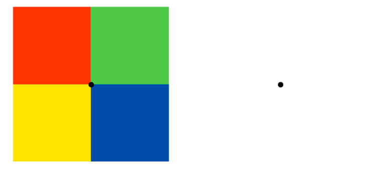
Rémanence visuelle et opposition de couleurs. Fixer le point noir central de l'image de gauche pendant 30s, puis déplacer son regard vers le point noir de droite. Observer que les couleurs perçues dans cette nouvelle image sont les complémentaires de celle du carré original. Comment l'expliquez-vous ?
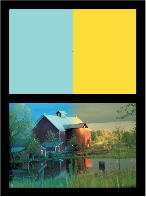
Adaptation chromatique locale. Fixer le point noir au centre de l'image du haut (entre les deux zones uniformes) pendant 30s environ, puis déplacer le regard vers le point blanc de l'image du bas. Observer que l'image du bas apparait beaucoup plus uniforme après cette adaptation.
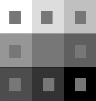
Contraste simultané Dans l'image suivante, les rectangles centraux ont tous le même niveau de gris. Comment expliquez-vous le fait qu'on les perçoivent différemment ?
2 Color images - Introduction
For the following exercices, you need either Matlab or Scilab.
You need first to download the file TP.zip, to unzip it so that you have a directory named TP containing two subdirectories scilab_src (which contains a few necessary scilab commands for loading and displaying images) and im (which contains images needed in the TP).
If you use Scilab you should add scilab_src to the path by typing (replacing PATH by the correct path…) :
getd('/PATH/TP/scilab_src');
The comments are indicated by '%'in Matlab and by '//' in Scilab.
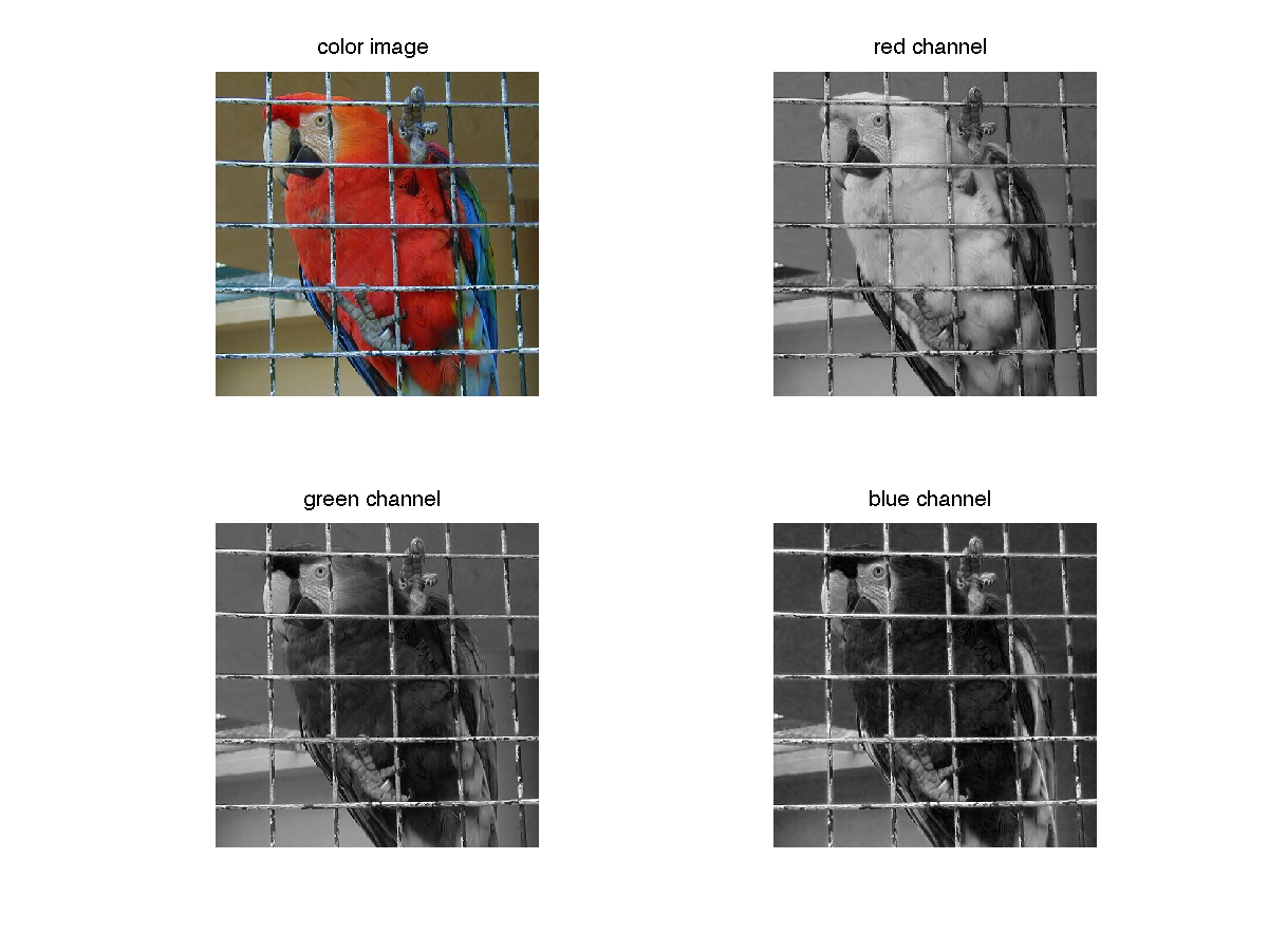
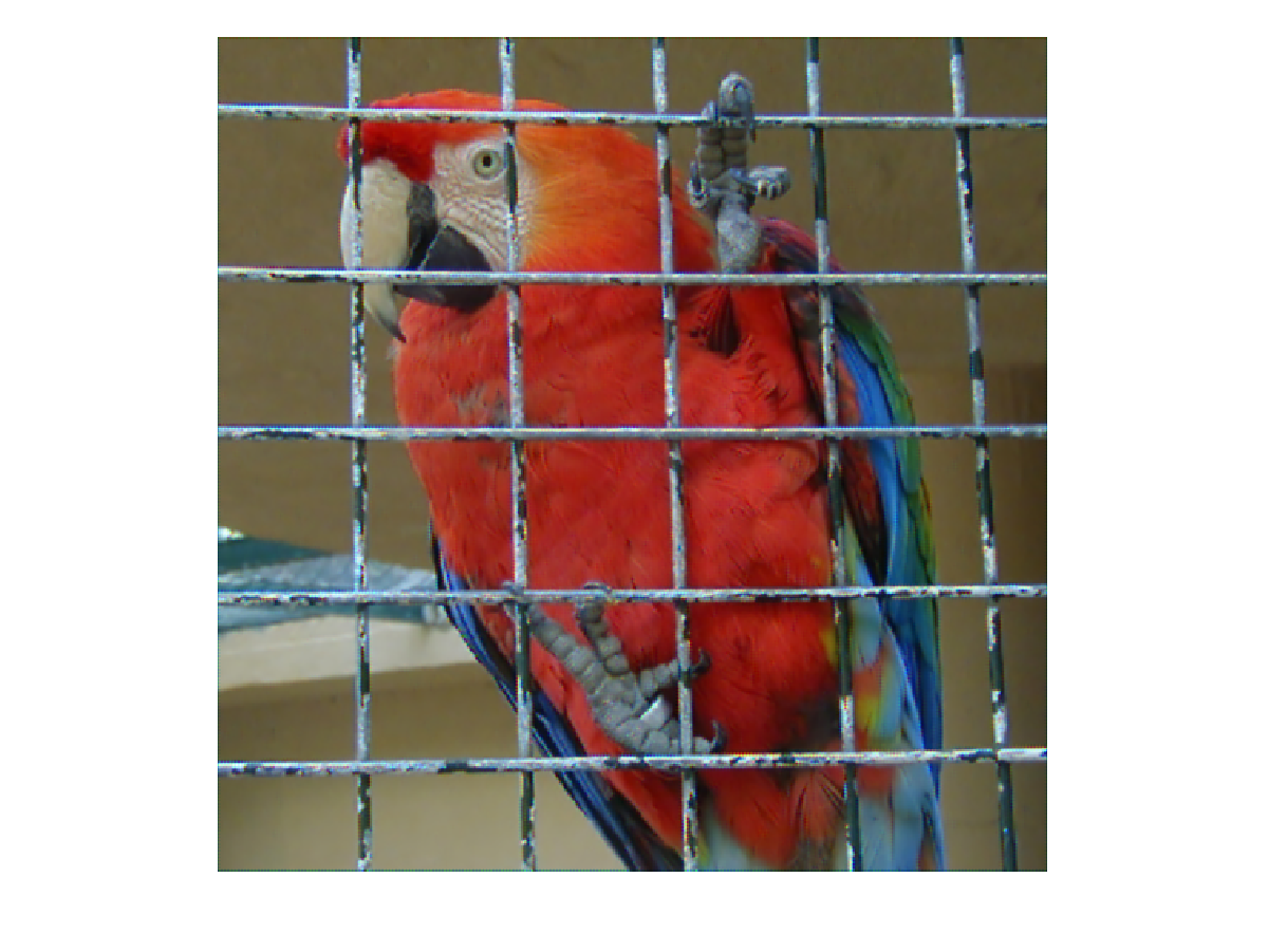
Load and display a color image. A color image \(u\) is made of three channels : red, green and blue. In Matlab and Scilab, a color image in \(\mathbb{R}^{N\times M}\) is stored as a \(N\times M\times 3\) matrix.
Scilab
imrgb = read_bmp_bg('im/parrot.bmp');  // load an image
[nrow,ncol,nchan]=size(imrgb);
ccview(imrgb); //display the color image
R = u(:,:,1); G = u(:,:,2); B = u(:,:,3);
fview([R,G,B]); // display the three channels
Matlab
imrgb = imread('im/parrot.bmp');  % load an image
[nrow,ncol,nchan] = size(imrgb);  % image size
figure;
subplot(2,2,1); imshow(imrgb,[]), title('color image')
subplot(2,2,2), imshow(imrgb(:,:,1),[]), title('red channel');
subplot(2,2,3), imshow(imrgb(:,:,2),[]), title('green channel');
subplot(2,2,4), imshow(imrgb(:,:,3),[]), title('blue channel');
It might be useful to convert the color image to gray level. This can be done by averaging the three channels, or by computing another well chosen linear combination of the coordinates R, G and B. The rgb2gray function in the image processing toolbox computes \(0.2989 * R + 0.5870 * G + 0.1140 * B\).
imgray = sum(imrgb,3)/3;
Before most computations, it is important to convert an image to double !!!
imrgb = double(imrgb);
Be careful with the function imshow(). If u is an image encoded in double, imshow(u) will display all values above 1 in white and all values below 0 in black. If the image u is encoded on 8 bits though, imshow(u) will display 0 in black and 255 in white. In order to scale u and use the full colormap, use the command imshow(u,[]).
3 Color spaces
3.1 Opponent spaces
Color opponent spaces are characterized by a channel representing an achromatic signal, as well as two channels encoding color opponency. The two chromatic channels generally represent an approximate red-green opponency and yellow- blue opponency. $$ O_1 = \frac 1 {\sqrt{2}} (R-G),\; O_2 = \frac 1 {\sqrt{6}} (R+G-2B),\; O_3 = \frac 1 {\sqrt{3}} (R+G+B)$$ Display the O1, O2 and O3 coordinates for different color images.
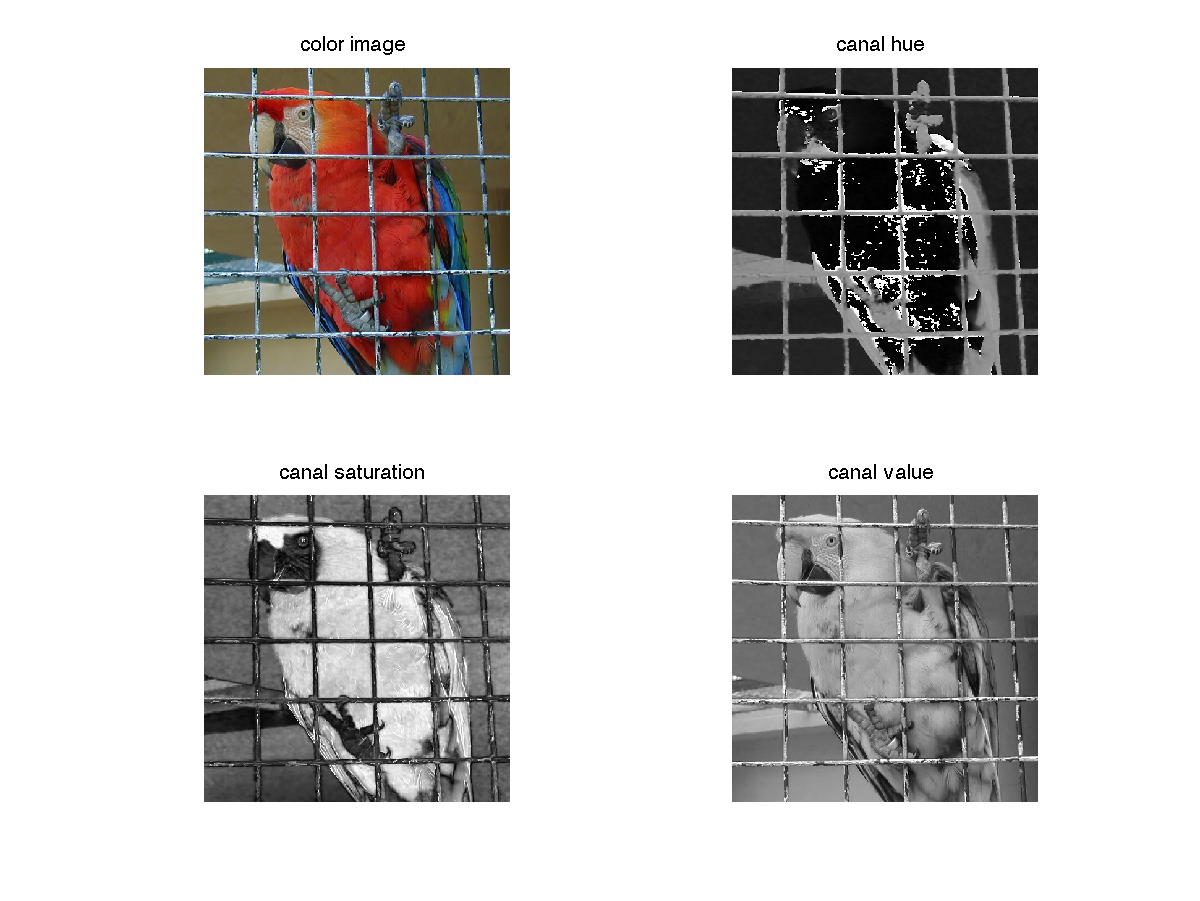
3.2 HSV/HSL/HSI spaces (Hue, Saturation, Value/Luminance/Intensity)
These colorspaces are obtained by a non-linear transformation of the RGB coordinates into polar coordinates. The luminance (or value V) corresponds to the vertical axis of the cylinder; the hue corresponds to the angular coordinate and the saturation to the distance from the axis. See https://en.wikipedia.org/wiki/HSL_and_HSV for more details.
The conversion from RGB to HSI boils down to $$ H=atan\left(\frac{O_1}{O_2}\right),\;S=\sqrt{O_1^2+O_2^2},\; I=0_3$$ The conversion from RGB to HSV is a little bit more complex, you can use the function rgb2hsv (rgb2hsv2 in Scilab) in order to compute it (the inverse transformation is hsv2rgb - hsv2rgb2 in Scilab).
imhsv = rgb2hsv(imrgb); % rgb2hsv2 in Scilab
- Display the H, S and V coordinates and the H, S and L coordinates for different color images.
- Observe the effect of JPG compression on the different
channels by applying the conversion on the images
parrotandparrotcompressed.

- Reconstruct and display the RGB image after the following
transformations :
- saturation reduction
- rotation of the hue channel
- gamma transformation on the luminance (\(x\mapsto x^\gamma\) with \(\gamma <1\)).
3.3 Space of perceived colors
Simulation of the set of monochromatic colors in RGB. The cone responses are approximated by Gaussian distributions.
Matlab
close all; clear all;
u=[0:1:1000];
r=exp(-(u-440).^2/(2*40^2));
g=exp(-(u-540).^2/(2*40^2));
b=exp(-(u-570).^2/(2*40^2));
figure; plot3(r(380:700),g(380:700),b(380:700),'kd');
Scilab
u=[0:1:1000];
r=exp(-(u-440).^2/(2*40^2));
g=exp(-(u-540).^2/(2*40^2));
b=exp(-(u-570).^2/(2*40^2));
figure; param3d1(r(380:700),g(380:700),list(b(380:700),-1));
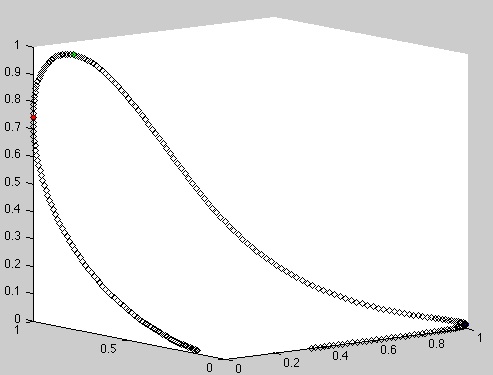
- Maxwell triangle : display the same curve after normalization of \(r\), \(g\) and \(b\) by the sum \(r+g+b\).
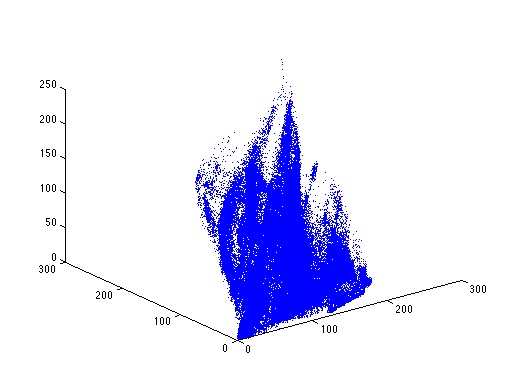
4 Color distributions and color quantization
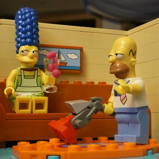
Display the color distribution of an RGB image as a 3D point cloud.
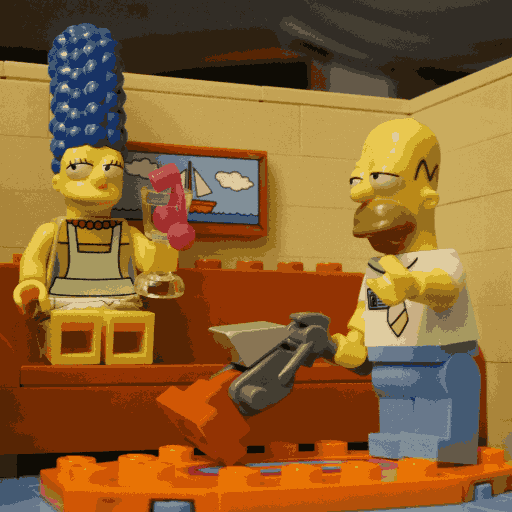
Matlab
u = double(imread('simpson512.png'));
[nr,nc,nch] = size(u);
rgb = reshape(u,nr*nc,nch);
plot3(rgb(:,1),rgb(:,2),rgb(:,3),'.');
Scilab
u = double(imread('simpson512.png'));
[nr,nc,nch] = size(u);
rgb = matrix(u,nr*nc,nch);
figure; param3d1(rgb(:,1),rgb(:,2),list(rgb(:,3),-1));
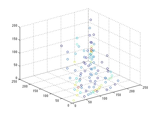
The point cloud is too dense for vizualization. A solution is to perform clustering on the point cloud before displaying it. The command 'scatter' permits to display the point cloud with colors based on the weights of the points.
Matlab
K = 100;
[IDX,C] = kmeans(rgb,K,'Start','sample');
h=zeros(K,1);
for i=1:K
    t = find(IDX==i);
    h(i) = length(t);
end
scatter3(C(:,1),C(:,2),C(:,3),[],h);
Color clustering can be used for color image quantization (\(K\)-means boils down to Lloyd-Max quantization in 1D).
v = C(IDX,:);
uquantif = reshape(v,nr,nc,3);
imshow(uquantif,[]);
- Add a gaussian white noise to \(u\) before the quantization to perform color dithering.
5 White Balance
5.1 White point
Assume that a light source has a constant spectral density on the range of wavelengths \([a,b]\), i.e $$ f(\lambda) = \frac{1}{b-a}\mathbf{1}_{[a,b]}.$$ What is the spectral density of this light source expressed as a function of frequency instead of wavelength ? Recall that frequency and wavelength of a light source are related by \(\nu = \frac c \lambda\), with \(c\) the light speed. What can we deduced on the possible definition of a white light ?
5.2 White balance algorithms
The chromaticities of objects in a scene
are highly dependent on the light sources. The goal of the white
balance algorithms is to estimate the color \(e = (e_R,e_G,e_B)\) of the
illuminant and to globally correct the image using this estimate so
that it appears as if taken under a canonical illuminant, by
computing
$$R= \frac{R}{e_R},\; G= \frac{G}{e_G}\; B=\frac{B}{e_B}.$$
In this exercice, we propose to code and test some famous white balance algorithms on the image moscou.bmp.
- White patch.
The White-Patch assumption supposes that a surface with perfect reflectance is present in the scene and that this surface correspond to the brighter points in the image. This results in the well-known Max-RGB algorithm, which infers the illuminant by computing separately the maxima \((R_{max},G_{max},B_{max})\) of the three RGB channels : $$e_R= \frac{R_{max}}{255},\; e_G= \frac{G_{max}}{255}\; e_B=\frac{B_{max}}{255}.$$
- Grey world.
A very popular way to estimate illuminant chromaticities in images is to assume that under a canonic light, the average RGB value observed in a scene is grey. This assumption gives rise to the Grey-World algorithm, which consists in computing the average color in the image and compensating for the deviation due to the illuminant, i.e. $$e_R = \frac{\int R(x)dx)}{128}, e_G = \frac{\int G(x) dx}{128}, e_B = \frac{\int B(x) dx}{128}.$$
- Shades-of-gray.
The Gray-World algorithm was generalized into the Shades-of-Gray algorithm by adding the Minkowski norm p: $$e_R = \left(\int R^p(x)dx\right)^{1/p}, e_G = \left(\int G^p(x)dx\right)^{1/p}, e_B =\left(\int B^p(x)dx\right)^{1/p}.$$
- General Gray-world
The previous algorithm is extended by smoothing locally the three channels by a Gaussian filter of standard deviation \(\sigma\).
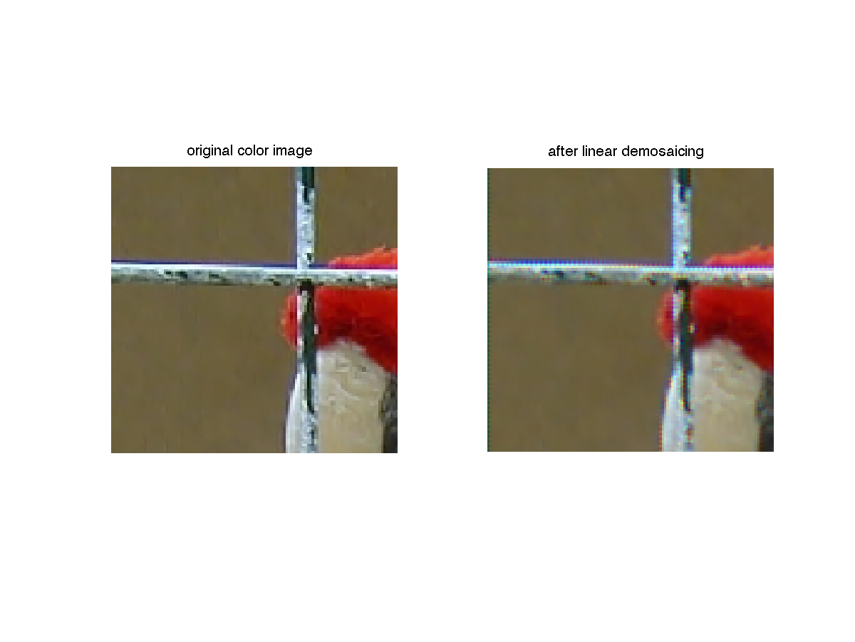
6 Demosaicing
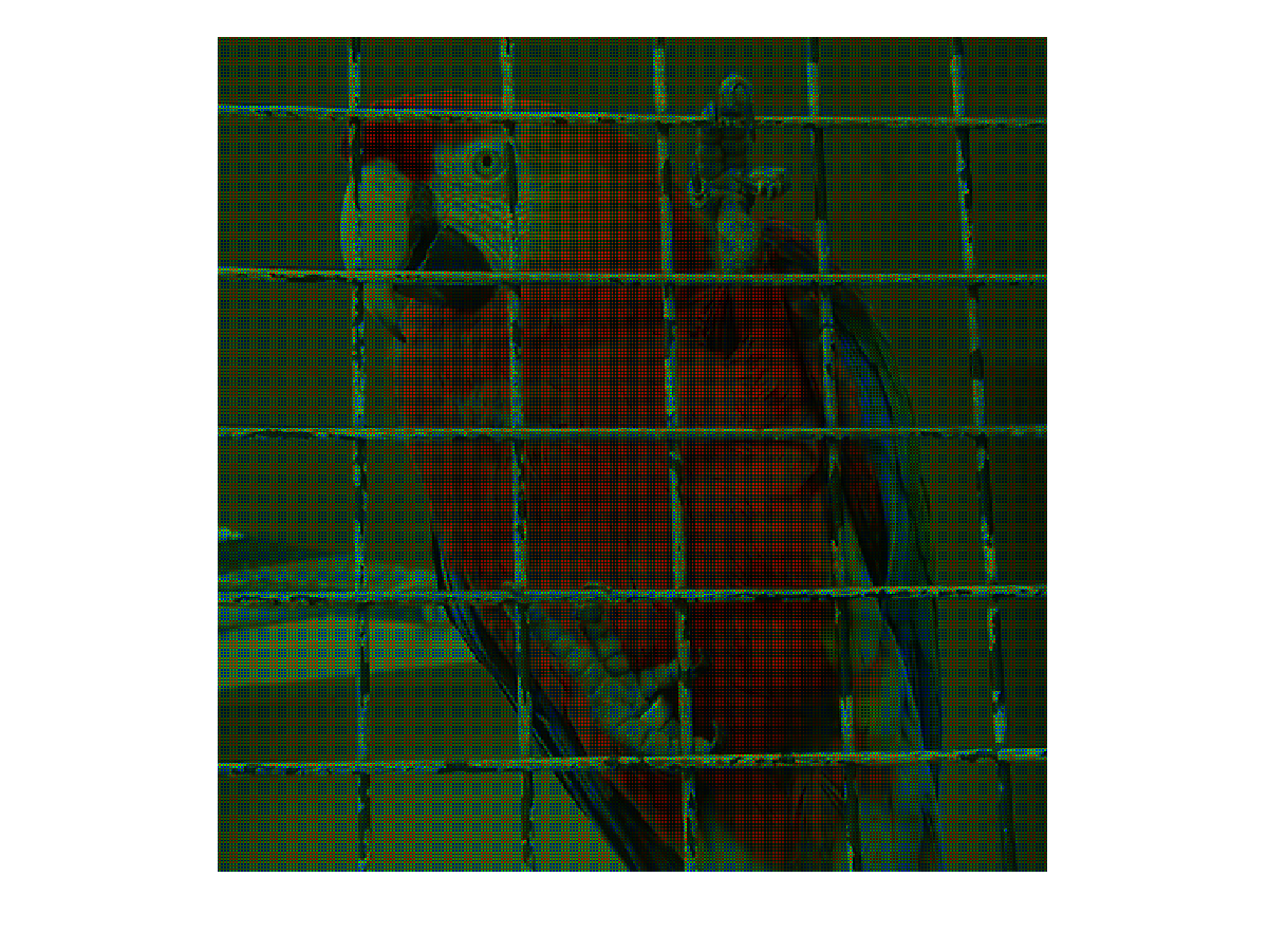
The following exercice can be done with parrot.bmp or lighthouse.bmp.
We first create a RAW image from the image imrgb. A each pixel, only one channel is known
(red, green or blue), follwing the Bayer CFA. Remind that the bayer
CFA has the following structure :
| R | G | R | G | ||||
|---|---|---|---|---|---|---|---|
| G | B | G | B | ||||
| R | G | R | G | ||||
| G | B | G | B |
bayer = zeros(nrow,ncol,nchan);
raw(1:2:nrow,1:2:ncol,2)   = imrgb(1:2:nrow,1:2:ncol,2);
raw(2:2:nrow,2:2:ncol,2)   = imrgb(2:2:nrow,2:2:ncol,2);
raw(1:2:nrow,2:2:ncol,1)   = imrgb(1:2:nrow,2:2:ncol,1);
raw(2:2:nrow,1:2:ncol,3)   = imrgb(2:2:nrow,1:2:ncol,3);
Display the resulting image.
imshow(raw,[]); %ccview(raw); in Scilab
Now, in order to retrieve the original image, we can try to interpolate each channel, for instance by bilinear interpolation.
R = raw(:,:,1); G = raw(:,:,2); B = raw(:,:,3);
G = G+conv2(G, [0 1 0; 1 0 1; 0 1 0]/4, 'same'); % Interpolation of the green channel at the missing points
B = B+conv2(B,[1 0 1; 0 0 0; 1 0 1]/4, 'same');
B = B+conv2(B,[0 1 0; 1 0 1; 0 1 0]/4, 'same'); % Interpolation of the blue channel at the missing points
R = R+conv2(R,[1 0 1; 0 0 0; 1 0 1]/4, 'same');
R = R+conv2(R,[0 1 0; 1 0 1; 0 1 0]/4, 'same'); % Interpolation of the red channel at the missing points
output(:,:,1)=R; output(:,:,2)=G; output(:,:,3)=B;
Display the result
imshow(output,[]); % ccview(output) in Scilab
Zoom on the metal grid and observe the mosaic artifacts. How can you explain them ? In order to understand these artifacts, create a white image with a black square in the first top quarter and apply the same process (RAW image creation and demosaicing by bilinear interpolation of each channel). Comment the result.